#
Tracking model performance
After a successful training, you can go to a detailed view of the model to check its statistics or make additional conversions.
![]()
The top section displays basic information about the model, such as:
- Name of the trained model
- Framework used
- Pretrained model selected
- Configuration
- Creation date
In the Statistics section you can see general information about the trained model:
![]()
Statistics are calculated on the basis of accuracy/loss functions. Their detailed description can be found in the documentation of the chosen framework.
- Accuracy - average model precision
- Loss - model loss
- Training time
#
Classification accuracy
#
Keras and PyTorch frameworks
For the Keras and PyTorch classification models, the following measures of accuracy ratings are calculated for each class:
- Precision - TP/(TP + FP)
- TP - True Positive, i.e. the number of pictures correctly attributed to a given class
- FP - False Positive, i.e. the number of pictures incorrectly attributed to a given class
- Recall - TP/(TP + FN)
- FN - False Negative, i.e. the number of pictures incorrectly attributed to a different class
- F1-score (2 * precision * recall / (precision + recall))
![]()
You can then analyze interactive graphs showing the change in Accuracy/Val Accuracy and Loss/Val Loss values against epochs.
![]()
A Confusion Matrix is another element that helps assess whether your model has been trained correctly.
CM is an N×N matrix, where the columns correspond to the correct decision classes and the rows correspond to the recognitions of the learned model. The number at the intersection of the column and row corresponds to the number of images from the column class that were assigned to the row class by the classifier.
![]()
Efficiency percentage range for diagonal cells (the range is inversed for non-diagonal cells):
- Very low efficiency [0% - 20%]
- Low efficiency [21% - 40%]
- Medium efficiency [41% - 60%]
- High efficiency [61% - 80%]
- Very high efficiency [81% - 100%]
The diagonal cells represent correct recognitions. For example, the current model recognized 85.71% of the horse photos correctly, which is in the very high efficiency range (80-100%), so this cell has been colored green.
Each row adds up to 100%. For example, the cells on the left represent photos where tigers were recognized as cats, dogs, goats, horses and lions. These cells have been colored green because of the range inversion. The lower the number of misrecognitions, the more effective the model is.
In simple words: the more green cells in the matrix, the better the trained model. For each cell that is not green, the overall efficiency of the model decreases according to the percentage range shown in the cell (and the corresponding colors). The model is completely useless if the matrix is all red.
![]()
![]()
#
Detection accuracy
#
Darknet framework
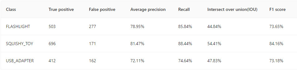
For the Darknet detection model, for each class we can extract the following statistics:
- True positive - i.e. the number of detections correctly recognizing a given class
- False positive - the number of detections that falsely recognize a given class
- Average precision - TP/(TP + FP)
- Recall - TP/(TP + FN)
- Intersect over union = area of overlap / area of union
- Area of overlap - area of overlap actual and predicted label
- Area of union - area of union of the actual and predicted label
- F1-score - (2 * precision * recall / (precision + recall))
#
Tensorflow framework
For the Tensorflow detection model, for each class we can extract the following statistic:
- Average precision - TP/(TP + FP)
![]()
You can then analyze the interactive graphs that show the change in Precision and Loss values against every hundredth iteration.
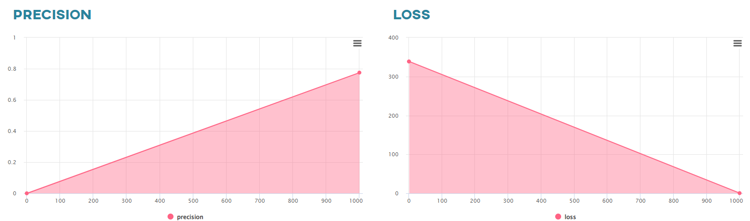
The Precision value is calculated after the Burn In process is completed.